Mathematical Models and their Application in Cancer Growth

Fuad Mugarab-Samedi*, Sahbaz Heir and Saboor Ul-Bashar

Faculty of Mathematics, University of Calgary, Canada

*Corresponding Author: Fuad Mugarab-Samedi, Faculty of Mathematics, University of Calgary, Canada.

Received: April 28, 2021; Published: June 30, 2021

Abstract

  Cancer is defined as a collection of related diseases. The common prevailing factor in all different forms of cancer is that the cancer cell begins to divide without any control and invades nearby tissues, spreading through the lymph system [1]. Although solutions are found for restraining further spread or eliminating diseased cells, most of the methods fail to predict the early signs of such an occurrence. A useful catalyst utilized by specialists is using variant forms of differential equations, particularly ordinary differential equations (ODE's). By using ordinary differential equations, such as the Malthusian model and the Gompertzian model, and state which method would be more efficient. Models such as the "Gompertzian growth curve" helps us visualize the growth rate of a cancerous cell. The Gompertzian model describes the cancer growth as a curve, which then has an almost exponential growth rate followed by a slower growth rate, which reaches a plateau as tumors grow larger [2]. Finally, we will use Matlab to code a graph that describes the mathematical growth models. In this paper, we will reveal how we can use ordinary differential equations to solve cancer growth spread, while also touching on some other models.

Keywords: Cancer; Bio-organism; Gompertzian Model

Introduction

  The history of Mathematics is not a boring one but rather interesting. Math has evolved constantly with our curiosities, benefiting and explaining the laws of the universe while also aiding us in understanding our bodies. One of the many ways Math helps us is explaining tumor growth, specifically cancerous ones, in bio-organisms such as ourselves and many other species on our planet.

  In this paper, we will be discussing tumor growth and how it spreads as abnormal cell division of cancer. We will define this growth using two specific models, Malthusian and Gompertz. Furthermore, we will observe how the Gompertz model is more competent in measuring tumor growth for long periods when compared with the Malthusian model. We will demonstrate this by plotting Tumour growth curves for both models to accurately capture the growth rate of the tumor volume.

What is cancer?

  Our bodies are composed of countless cells that die and get replaced by new ones. These new cells are derived from the existing cells within our body, as the previous ones complete their cycle the new cells take their place. However, on rare instances, these cells divide without any restraint causing an abnormality within our bodies which we call “cancer". The National Cancer Institute defines cancer as various and similar diseases that affect the human body and different bio-organism [3].

Figure 1: A visual representation between Normal Cells and Cancer Cells.

  To understand cancer, we must grasp an idea of a cell and a cell cycle. All cells go through physiological cell cycle: the growth and asexual reproduction of a cell (process consists of interphase, which is then followed by the division of a cell by prophase, metaphase, anaphase, and telophase). Cancer cells also undergo this cycle, but their behaviour is unlike that of normal cells; they grow and divide in an uncontrolled manner, invading normal tissues, organs, and eventually spreading throughout the body. It is hard to pinpoint the etiology of cancer, since it can occur from a wide range of variables, from genetic to environmental. The genetic alterations that contribute to cancer tend to affect three main types of genes; proto-oncogenes, tumor suppressor genes, and DNA repair genes. These genes are often called as the “drivers" of cells as they are responsible for repairing and maintaining regular cell growth and division. But once these genes are corrupt, they become what are known as cancer drivers". Once these cells begin to multiply, they can either spread throughout the body or stay put in one part.

  Cells that form tumors spread around various parts of the body are known as malignant tumors [4]. Similarly, cancer cells that do not spread are known as benign tumors [5]. Benign tumors usually do not spread or invade nearby tissue, thus when you remove them, they usually do not come back. On the other hand, the malignant tumors will spread and invade nearby tissue.

  Cancer is one of the leading causes of death in all age groups among males and females. The Canadian Cancer Statistics released a publication in 2017 stating that “During an average Canadian lifetime, nearly 1 in 2 Canadians will be diagnosed with cancer, and 1 in 4 will die from the disease" [6]. But given how disastrous the nature of this disease is, there has been a tremendous amount of financial and human resources invested into funding some form of a prevention or resolution for it. With a number of breakthroughs with the help from various fields in medicine and science, every day we get one step closer to our goal.

Malthusian model Background

  During the 18th and 19th century, philosophers considered whether the humanities population would never seize to grow. Many believed that populations would grow indefinitely. However, an economist, Thomas Malthus (1766-1834), created a model, which would state otherwise. In 1798, Malthus anonymously published his first book titled “An Essay on the Principle of Population" [7]. In this book, the data and information that was provided received wide notice, as it challenged the way of thinking at that time. With this growth model, Malthus proved that the population growth will outgrow the rate of production. Thus, the human population cannot grow forever if it outgrows the rate of food that would have to be produced. Even though this model has been utilized in Economics, scientists started to operate Malthus' principles in the medical field. The Malthusian growth model comes from the Malthusian growth law. Stephen W. Goode and Scott A. Annin describes this as a “Mathematical model of a population growth that is obtained by assuming the rate of increase of the population at any time, is proportional to the size of the population at that time" in their book Differential Equations and Linear Algebra, a custom edition for Purdue University [8]. Given the following definitions, we can apply it in tumor growth.

Malthusian growth model

  The following definitions for generating the growth model are directly from the textbook provided by Purdue University. By understanding the variables and how to solve for the growth model, we can then use it to solve for tumor cell growth.

  Suppose that P(t) describes some population of a given area at time t. Deriving P(t), we get dP/dt = kP where we define k as a positive constant. Solving for P(t), we get where P₀ is the P(t) = P₀e^kt population at the start (at t = 0).

The amount of time it could take for a cell to double in size can be referred to as the doubling time, we will refer to as td. So looking at the Malthusian growth model, we get

P(t_d) = 2P₀ = P₀e^kt_d--------- (1)

Rearranging, we acquire kt_d = ln(2) which gives the doubling time to be

t_d =1/k ln(2)

  With this knowledge in mind, we can look at how Malthusian is used in modeling cancer growth. By setting our P variable to represent the population of cancer cells, then we can assume that P₀ would be the initial sum of cancer cells at time t = 0, and thus determine the doubling time td of the cancer growth/regression rate over time t. This is a very helpful method for specialists who can then derive an appropriate time as well as dosage of medication, maximizing its effect in reducing further tumor growth.

Example of cell growth using Malthusian

For the next part, we create an example of a cell growth in a tumor using the Malthusian model. Suppose that a number of cancer cells are developing at the rate that is proportional to the value present. In 2 hours, the number of cells has increased from 400 to 3600.

First we determine the number of cells present 12 hours later.

Secondly, determine the doubling time.

Solution a):

P(t)=P_O∙e^kt ------- (1)

Where the time t is measured in hours. By setting t = 0, P₀ = 400, then

P(t) = 400 ∙ e^kt---------- (2)

Now, if P(2) = 3600, then by rewriting the equation above, we get

3600 = 400 ∙ e^2k----(3)

Thus, the solution for k is given as k = ⅟₂ ln(9) = ln(3). Therefore,

P(t) = 400 ∙ e ^{t ln(3)} -----------(4)

And we can conclude that the number of cells present after 12 hours is

P(12) = 400e² 4 ln(3) = 212, 576, 400.

Solution b):

Given that doubling time for Malthusian is t_d = 1⅟k ln(2), then the doubling

time of the tumor to growth is t_d = ⅟_ln(3) ln(2) = 0:630929860 ∙60(minutes) =37.86 minutes.

Drawbacks to malthusian

  The Malthusian model does come with its flaws because when creating it, Malthus himself knew that it had inefficiencies. As mentioned above, cancer cells have a high growth rate, eventually over time, the population of those cells begin to regress. This happens due to multiple reasons, such as the number of cells in a tumor being at its maximum capacity or the initiation of cell spreading through the lymph nodes via metastasis. However, the Malthusian Model works under the assumption that the rate of increase of a population at any time, is proportional to the size of that population at that time. Since the Malthusian model is unbounded, it is essentially only good for modelling short term projections.

  Rushton Parker, a professor of Surgery in Liverpool University published a medical journal stating the drawbacks for the Malthusian model [3]. In his research, he affirmed that the model does not account for the long term growth such as in malignant tumors, since their growth rate regresses over time. Thus the model is only useful for benign tumors. But when modeling cancer growth, it is critical to account for all variables. Since Malthusian method does not account for malignant tumors, we will further investigate some other models that exist.

Gompertz model Background

  The Gompertzian model is named after the English mathematician Benjamin Gompertz. It describes the growth and decay rate of bio-organisms such as plants, cells and bacteria, at the beginning and the ending of a time period. This model is very commonly used in medicine as stated in a medical journal by Kathleen M. C. Tjorve and Even Tjorve “The Gompertz model is well known and widely used in many aspects of science. It has been frequently used to describe population growths, such as the number of bacteria and cancer cells" [9].

Gompertzian growth model

In order to understand the Gompertz model, we first need to understand the Gompertz function. The function is given to us as

V (t) = ke^{-ln( k/V0)e -αt}--- (1)

Where,

V (t) = Cancer cell population at a given time t,

α = Constant that defines the rapid increase of cancer cells,

k = Carrying capacity.

Unlike Malthusian, the Gompertz model has a natural logarithmic function which allows it to be bounded. This allows the model to be useful for modelling long term growth rates of a population such as cancerous cells. The carrying capacity is the average volume of cells in a given system, where they can sustain themselves given their environmental constraints. These constraints usually mean the amount of minerals or nutrients that are available for those cells so they may endure.

The Gompertz growth is given by dV/dt = αln(k/_{V (t)} )V (t) where dV/dt is the constant rate of change in the population growth over time. This change can either be positive or negative, depending on whether the growth rate of cells is increasing or decreasing. Due to the constant change of the tumor growth rate over time, the Gompertz growth law must be derived.

Now, recall that dV/dt = αln(k/_V(t) )∙Vt. By moving dt and ln( k/_{V (t)} )V (t) respectively, we get

dV/ln( k/_{V (t)} )V (t)= α dt ----- (2)

Now, if we take the integral of the right hand side and left hand side we see that:

∫ dV/ln( k/_{V (t)} )V (t)= α∫ dt ---(3)

By using u-substitution on the left hand side, and simple differential methods on see that:

u = ln k/_{V (t)}= ln(k) - ln(V (t))----- (4)

Then,

du = -⅟_{V (t)}dV ----- (5)

Which can be re-written as,

dV = -V (t)du ---------- (6)

Now, by substituting what we got in (6) into our equation (2), we see that

∫V (t)du/u ∙V (t)= α∫dt ---(7)

ó-ln │u │ + C₁ = αt + C₂; (C₁ + C₂ = C)----(8)

ó-ln │ u │ = αt + C ---(9)

ó ln │ u │ = -αt – C----------(10)

ó│ u │=e^-αt-C -------- (11)

ó│ u │=±e^-αt-C -------(12)

ó u = ±e^-C ∙e^-αt = D ∙ e^-αt ----(13)

Where D = ±e^-C. Replacing our u substitution we have,

ó ln k/_{V (t)}= D e^-αt ------- (14)

Setting t = 0, we get V (0) = V₀, as well as e⁰ = 1. Thus,

=> D = ln k/V₀ -------- (15)

Which can be inferred as,

ó ln k/V (t)= ln k/V₀∙ e ^–αt ---- (16)

Simplifying the equation results into

ó V (t) = ke^{-ln( k/V0)e-αt} ------(17)

Differences between Malthusian and Gompertz

  One of the prevailing factors that makes Gompertz better, is the inclusion of ln k/V₀. The following natural logarithmic function modifies the growth rate, making it a better tool for observing the growth rate of tumors. It does so by making the model more bounded, unlike the Malthusian model.

  The Gompertz model, for example, shows that a tumor's rate of growth is greatest at the beginning stages, and then begins to regress substantially [10]. This is due to a high volume of competition for nutrients from cancer cells. Since the population increases, the amount of available nutrients decrease, which in turn causes the growth rate to slow down.

Graphing each model

  One way to get a better comprehension of the differences between the two models, is by graphing them. Using the data from the textbook “Advanced Statistics with Applications in R by Eugene Demidenko", we can create a graph that models the rate of growth for various tumors. When sampling these tumors, Eugene Demidenko did not enter the name for each different variant of a tumor. The reason this is essential, is because different tumors grow at different rates. For example; a tumor in the brain will grow at a much faster rate than a tumor in the lungs.

  A researcher, Daniela Mejia has coded a similar growth model using the data provided by Eugene Demidenko [11]. In her code, she visually compares the Malthusian and Gompertz Models. From Eugene Demidenko's book, Daniela first creates a simple graph that defines the growth curve for some tumor. From there, she generates both of the models, and by comparison, confirms the Gompertz accuracy. The graphs provided by Ms. Mejia will help in viewing the application of each model.

Figure 2 represents a growth curve of a single tumor cell where each plot point represents the Spheroid of the tumor cell calculated on a given day.

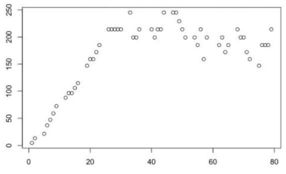
Figure 2: Growth curve of a single tumor cell.

Now, by inputting the Malthusian model in the following graph, we get figure 3.

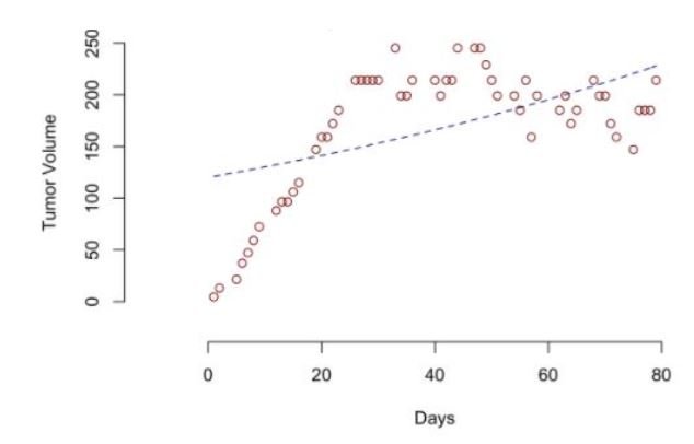
Figure 3

  It is clear that most of the points do not fall on the line itself meaning it doesn't accurately capture the growth rate of the tumor volume. Now, fitting the Gompertz model into figure 2, we see that it is sigmoidal in shape and fits the tumor cell growth much more accurately (Figure 4).

Figure 4

  Thus, the Gompertz model is accurate for both long and short tumor growths whereas the Malthusian model is only accurate for short term tumor growth as the Malthusian model is unbounded.

References

1. Definition of cancer - NCI Dictionary.
2. Rushton Parker. “Malthus's Law and Tumour-Growth”. British Medical Journal 1321 (1886): 778.
3. "What Is Cancer? - National Cancer Institute” (2015).
4. "Malignant Soft Tissue Tumors: Types, Symptoms Treatments”.
5. "Benign Tumors: MedlinePlus” (2020).
6. (2017, October 23). Canadian Cancer Statistics - Canada.ca (2021).
7. "Thomas Malthus - Biography, Theory, Overpopulation ... - Britannica” (2021).
8. "1.5 Malthusian Growth - Purdue Math” (2007).
9. Kathleen MC Tjørve and Even Tjørve. "The use of Gompertz models in growth analyses, and new Gompertz-model approach: An addition to the Unified-Richards family”. PLoS One6(2017): e0178691.
10. "Mathematical Models for Cancer Growth”. Callaix - Chemotherapy.
11. "Gompertz Curve - RPubs” (2019).
12. Linan Zhang., et al. “Computational analysis of the effects of matrix-degrading enzymes on cancer-cell invasion”. Journal of Applied Physics 112 (2012): 124704.
13. RA Gatenby and ET Gawlinski. "A reaction-diffusion model of cancer invasion”. Cancer Research24 (1996): 5745-5753.

Citation

Citation: Fuad Mugarab-Samedi., et al. “Mathematical Models and their Application in Cancer Growth”. Acta Scientific Cancer Biology 5.7 (2021): 35-41.

Copyright

Copyright: © 2021 Fuad Mugarab-Samedi., et al.. This is an open-access article distributed under the terms of the Creative Commons Attribution License, which permits unrestricted use, distribution, and reproduction in any medium, provided the original author and source are credited.