Erhan KAHYA1*, Fatma Funda ÖZDÜVEN2 and Yasin ASLAN3
1Tekirdag Namık Kemal University, Vocational School of Technical Sciences, Department of Electronics and Automation, Control and Automation Technology Programme, Tekirdag, Turkey
2Tekirdag Namık Kemal University, Vocational School of Technical Sciences, Department of Plant and Livestock Production, Greenhousing Programme, Tekirdag, Turkey
3Freelance Senior Software Developer, Tekirdag, Turkey
*Corresponding Author: Erhan KAHYA, Tekirdag Namık Kemal University, Vocational School of Technical Sciences, Department of Electronics and Automation, Control and Automation Technology Programme, Tekirdag, Turkey.
Received: September 10, 2024; Published: September 24, 2024
Citation: Erhan KAHYA., et al. “Yolov8 Based Recognition of Green Pepper Performance Comparison of Object Recognition Models and Training Processes". Acta Scientific Agriculture 8.10 (2024): 32-49.
Deep learning-based object recognition models are an important innovation in agriculture, especially in areas such as peppers classification and early disease detection. YOLOv8 models can provide high accuracy rates in recognizing green pepper varieties and diseases. In this study, the performance of different deep learning models from the YOLOv8 family in classification and detection systems was evaluated. Among the YOLOv8 models, four different versions are considered: YOLO Nano, YOLO Small, YOLO Medium and YOLO Large. The advantages and disadvantages as well as the suitable areas of application of each model were analyzed in detail. YOLO Nano is characterized by its low energy consumption and fast processing capacity, but has limited applications due to its low accuracy and sensitivity to noise. YOLO Small, on the other hand, offers balanced performance by providing high accuracy and mAP values. Thanks to its transfer learning capability, it can be effective in complex tasks but requires more power and memory. YOLO Medium offers balanced performance and provides high accuracy with a stable learning curve, but is characterized by moderate energy and memory consumption. The YOLO Large model has the highest accuracy and mAP values and is the most resistant to noise, but is limited by the highest energy and memory consumption. The YOLO Small model was identified as the most suitable option as a result of the evaluations. This model offers a balanced solution in terms of performance and speed while remaining at a reasonable level in terms of energy efficiency and memory consumption. It was found to perform successfully in real-world applications and allows for quick customization with transfer learning.
Keywords: Deep Learning, YOLO, Identification, Classification, Green Pepper
The green pepper plant is a vegetable that is widely grown in our country and around the world. It is rich in vitamins and is considered very valuable, especially in terms of vitamin C [1]. In our country, the cultivation of sweet green pepper is widespread in the Aegean, Marmara, Mediterranean, Southeastern Anatolia and Black Sea regions. In the Aegean and Marmara regions, pepper is grown for fresh consumption or for processing in the food industry, while in the East and Southeast Anatolia regions, most of the pepper production, especially powder and chilli flakes, is consumed in the domestic market and a small proportion of 2% is exported. Pepper is exported in dried form, as chilli flakes and chilli powder, frozen, roasted, pickled, pickled, as an additive in various foods or canned and contributes significantly to the economy of our country [2]. It is reported that the total protein and sugar content of pepper fruits is 16%-18% and 20%-40% respectively. In addition, chilli fruits contain oil, pigments, protein, cellulose and various minerals. Many species of the Capsicum genus contain considerable amounts of B, C, E and provitamin A (carotene). Peppers, which are very rich in vitamin C, can contain up to 340 mg/100 g of vitamin C, depending on the variety. Pepper, which differs from other species in its biochemical structure, is a powerful antioxidant and an important vegetable that should be consumed for the prevention of cardiovascular diseases and for a healthy lifestyle due to the cortonoid and various phytochemicals it contains [3]. Chilli is also used in the food industry in various ways. Chilli oil, one of the applications of pepper, is used in the food industry as a spice and flavouring agent. Chilli oil is mainly used in Chinese cuisine as a traditional spice oil and can enrich the dining experience by adding a unique flavour and aroma to dishes [4]. The production and harvesting of pepper is one of the most important issues in the agricultural sector. Although the green pepper plant is generally grown in the open field, production is carried out under greenhouse conditions in the off-season [5]. The use of modern technologies in the harvesting and production of pepper is also an important issue. Pepper cultivation is usually done in gardens of 2500-3000 m² and drip irrigation method is often preferred [6].
Deep learning is a branch of machine learning (ML) in which artificial neural networks (algorithms that function like the human brain) learn from large amounts of data. Deep learning is supported by layers of neural networks, which are algorithms that are generally modelled on the way the human brain works. Training with large amounts of data is used to configure the neurons in the neural network. The result is a deep learning model that processes new data after it has been trained. Deep learning models receive information from multiple data sources and analyse this data in real time without the need for human intervention. In deep learning, graphics processing units (GPUs) are optimised for training models because they can perform multiple calculations simultaneously [7]. Deep learning enables the automatic learning of higher-level features, in particular thanks to the multi-layered structure of neural networks. In this way, deep learning has become an effective tool for extracting meaningful information from large data sets, especially in areas such as medicine, image processing and industrial applications. Developments in the field of deep learning have accelerated mainly due to the contributions of large technology companies (Amazon, Google, Microsoft, etc.) [8].
Research on how deep learning can be used for sustainable development in education shows that deep learning can improve students' thinking skills and increase learning outcomes [9]. Deep learning models are also used in clinical applications in medical fields such as radiation oncology to support clinicians in their daily work and predict treatment outcomes [10]. Deep learning is used in many areas. Application examples include areas such as image processing, signal detection and optical flow. The SPD matrix representation based on spectral convolutional features is effectively used for signal detection with deep neural networks [11]. Most of the modern strategies developed for optical flow consistently incorporate deep learning architectures [12]. Deep learning has a wide range of applications in medicine, agriculture, energy, information technology and many other fields. This method is successfully used as an effective tool for solving complex problems, analysing data and pattern recognition. Classification, which is one of the areas of deep learning, has been widely used in disease detection and determining crop criteria in many agricultural products. [13] classified images of apple varieties using Convolutional Neural Networks (CNN) and achieved positive results. With the use of deep learning models, important steps are being taken in areas such as monitoring the growth status of plants, diagnosing diseases and monitoring plant health. In this way, robotic harvesting systems can closely monitor the health status of plants and intervene when necessary [14]. With the use of deep learning techniques, many operations such as irrigation, fertilisation, spraying, weeding of agricultural products can be performed by autonomous systems [15]. This increases productivity in agriculture, reduces labour and ensures automation. Deep learning also plays an important role in pepper classification systems. These systems usually contain neural networks developed for object recognition tasks and are used to classify images into relevant classes [16]. The proposed architectures show overall superior performance at high signal-to-noise ratios and significantly reduce training and prediction times, while significantly improving classification accuracy at high signal-to-noise ratios [17]. The integration of the redundancy module, which enables deep fusion of deep and shallow features, improves the effectiveness of the features and makes them useful for typical product classification [18]. Studies have aimed to extract richer features and increase the complexity of the model by increasing the complexity of extended and deep neural networks to combine multiple features [19]. These methods combine the advantages of stacked autoencoder networks to reduce the amount of data and convolutional neural networks for classification [20]. Hierarchical structures have also been used, allowing features at multiple levels to be combined with each other to express complex data patterns [21]. Furthermore, in a study by Taguchi., et al., an automated mushroom harvesting system was developed with a combination of robotics, virtual reality and artificial intelligence technologies. This system consists of five mechanisms such as data collection, mushroom recognition, harvesting target selection, automatic harvesting and unit movement [22]. Such integrated systems have significant potential to increase productivity and optimise harvesting processes in agriculture. [23] investigated the use of flexible piezoelectric nanogenerators made of CuInP2S6 for biomechanical energy harvesting and speech recognition applications. This study showed that the polarised CIPS-based PENG produced a short-circuit current of 760 pA at a strain rate of 0.85%, which was 3.8 times higher than that of the unpolarized CIPS-based PENG. Such technologies can also be used in agriculture by enabling innovation and efficiency gains in the field of energy production.
The aim of this study is to investigate the usability of deep learning based object recognition models in agricultural applications. In particular, the most suitable model for agricultural automation will be identified by comparing the performance of the Nano, Small, Medium and Large models of the YOLOv8 family. In this context, studies on the classification and disease detection of various agricultural crops such as peppers, tomatoes and strawberries were evaluated and the accuracy and efficiency performances of the YOLOv8 models at different difficulty levels were analysed. The study aims to contribute to the improvement of agricultural productivity and early disease detection by considering critical factors such as the complexity of the dataset, the difficulty of the tasks and the hardware capacity of the devices in the model selection.
Pepper (Capsicum annuum) is an important agricultural product for our country and is one of the most important vegetables in the nightshade family (Solanaceae) and is consumed both raw and cooked in the human diet. Peppers are grown in almost all regions of our country, both under cover and in the open field. One of the most important factors influencing the quality and shelf life of peppers after harvest is harvesting at the right time. The timing and environmental conditions from harvest to consumption are important in determining the ripeness of the chilli fruit to be harvested. Harvesting at the wrong time has many negative effects. green pepper fruits should have the desired colour, aroma and flavour at the appropriate harvest maturity, or if they will continue to have these characteristics after leaving the plant, they should be able to meet the maturity criteria required to reach eating maturity. For some harvested green pepper varieties, the fruit will continue to ripen depending on the environmental conditions (temperature, weather, etc.). Peppers are usually harvested manually by observing the colour and ripeness stage of the plant. In industrial production, harvesting is done mechanically [24]. For the study, 900 photos from Roboflow's image libraries were used as a training and test set. 700 of these photos were used in the training group and 200 in the test group. Examples of the images taken can be found in Figure 2. For the verification of the test set, 60 photos from the greenhouse of Tekirdag Namik Kemal University of Technical Sciences and the greenhouse of Tekirdag Naip Village were used. The pictures of the test set were taken with a Nikon D3100 camera. The camera resolution is 1920 x 1080 and the image format is jpeg. The pictures were taken at a distance of 0.5 cm from the pepper fruits. The pictures were taken between June 2024 and July 2024 and the pictures from the greenhouses can be seen in figure 1,2.
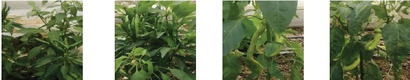
Figure 1: Test data (original).
![Figure 2: Training set data (Anonymous [25-30]).](https://actascientific.com/ASAG/images/ASAG-08-1414_figure2.png)
Figure 2: Training set data (Anonymous [25-30]).
YOLOv8 is the latest version of the YOLO series of real-time object detectors. Based on previous YOLO versions, YOLOv8 is faster and more accurate while providing a unified framework for training models to improve performance.YOLOv8 is a state-of-the-art object detection algorithm that outperforms many other object detection algorithms in terms of both speed and accuracy. [31] Building on the advances of previous versions, it offers users new features and optimizations that make it an ideal choice for a variety of object detection tasks in a wide range of applications [32]. Figure 3 shows the YOLOv8 backbone structure.
![Figure 3: YOLOv8 backbone structure [33].](https://actascientific.com/ASAG/images/ASAG-08-1414_figure3.png)
Figure 3: YOLOv8 backbone structure [33].
YOLOv8, the latest version of the You Only Look Once (YOLO) series of object detection models, represents a significant advance in real-time object detection technology. Released by Ultralytics in January 2023, YOLOv8 is designed to improve detection capabilities in a variety of applications, including agriculture, surveillance and industrial inspection [34]. This model integrates a more efficient architecture that balances speed and accuracy, making it suitable for use in resource-constrained environments such as embedded systems and unmanned aerial vehicles (UAVs) [35]. One of the highlights of YOLOv8 is its optimised architecture that enables better detection of small objects, a common challenge in many practical applications. Research shows that YOLOv8 is specifically designed to detect small objects using techniques such as automatic bounding box size optimization [36]. This feature is particularly useful in scenarios such as UAV aerial photography, where small targets are common and require precise identification [37]. In addition, studies have shown that YOLOv8 outperforms its predecessors by achieving higher F1 values and higher mean accuracy (mAP) in various test environments, demonstrating its robustness and reliability [38,39]. In the context of real-time applications, YOLOv8 is optimised for speed without compromising accuracy. A pruned version of YOLOv8 was able to significantly reduce inference time while maintaining a competitive average accuracy. This balance between speed and accuracy is crucial for applications such as CCTV surveillance, where timely detection can be critical [40]. The versatility of YOLOv8 has been demonstrated in various fields, including agriculture, where it has been used for early detection of drought in crops and identification of pests[41][42]. The model's ability to adapt to different data sets and application requirements underlines its potential as a state-of-the-art tool in precision agriculture and environmental monitoring. YOLOv8 stands out as a powerful and flexible framework for object detection that overcomes the challenges of real-time detection in various applications. Its improved architecture, focus on small object detection and optimization for speed and accuracy make it a valuable application in surveillance, agriculture and beyond.
Evaluation metrics such as precision (P), recall (R), average mean precision (𝑚 𝐴 𝑃 ) and frames per second (FPS) were used to comprehensively evaluate the performance of the model on the Glove dataset. The evaluation metrics used to comprehensively evaluate the performance of the model on the Glove dataset are: precision (𝑃 ), recall (𝑅 ), Average Precision (𝑚 𝐴 𝑃 𝑃 ), and Frames per Second (𝐹 𝑃 𝑆 ). These metrics are used to measure the accuracy, effectiveness and efficiency of the model in detail.
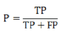
Precision (P): Precision measures the proportion of true positives among the model's positive predictions. It is calculated using the following formula
Here
TP (True Positives): Positive examples correctly identified by the model.
FP (False Positives): Examples that the model incorrectly identified as positive.
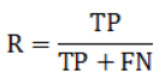
Recall (𝑅): Recall measures the rate at which the model correctly recognises positive examples. It is calculated using the following formula:
FN (false negatives): Positive examples that the model incorrectly identifies as negative.
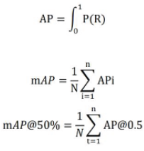
Average average precision (𝑚𝐴𝑃): The average mean precision is a summarized metric of precision at different recall values. It is calculated by averaging the average precision (AP) values for each class:
Here:
AP_i: Average precision for class i. N: Number of classes.
𝑚 𝐴 𝑃 @50% refers to the mean average precision with a threshold of 0.5 for the overlap across the union (IoU). This threshold is used to determine whether a predicted bounding box is considered a true positive or not. An IoU of 0.5 means that the overlap between the predicted bounding box and the ground truth box must be at least 50% for the prediction to be considered correct. The notation 𝑚 𝐴 𝑃 @50% denotes the average precision calculated with this IoU threshold and reflects the performance of the model in terms of precision and recognition with a moderate overlap.
Frames per Second (𝐹 𝑃 𝑆 ): Frames per second measures the processing speed of the model. It determines how many frames per second the model processes and indicates its computing power. It is calculated using the following formula:
Here:
T: Time required to process one image.
These metrics are used to evaluate the accuracy and efficiency of the model in detail, giving you a comprehensive understanding of the effectiveness of the model for the glove dataset.
![Figure 4: Trial Results (Anonymous [25-30]).](https://actascientific.com/ASAG/images/ASAG-08-1414_figure4.png)
Figure 4: Trial Results (Anonymous [25-30]).
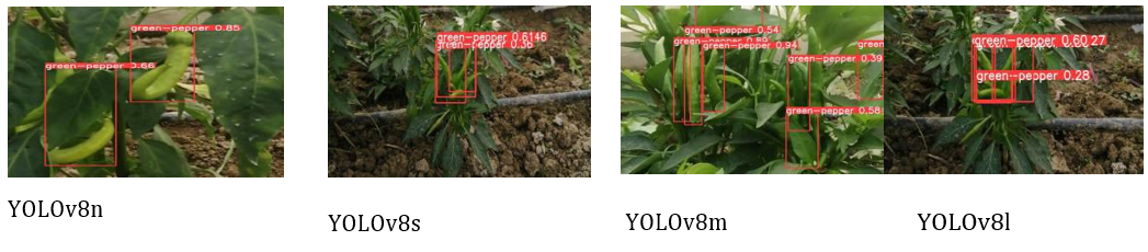
Figure 5: Trial Results (Original).
The confusion matrix is a basic metric for evaluating the performance of a classification model. This matrix visualises the correct and incorrect classifications of the model in detail. The confusion matrix consists of four main components: true positives (TP), false positives (FP), true negatives (TN) and false negatives (FN). These components are obtained by comparing the results predicted by the model for each class with the actual values.
Using these four components, the confusion matrix enables the calculation of performance metrics such as accuracy, recall, precision and F1 score. This matrix is an effective tool to determine in which classes the model is strong and in which classes it needs to be improved.
The normalised confusion matrix illustrates the proportions of correct and incorrect classifications for each class. This matrix shows in detail the proportions of correct classifications (true positives) and misclassifications (false positives and false negatives) by normalising the proportion of each class in the total predictions. The normalised confusion matrix provides a clearer assessment of the model's performance on a class-by-class basis and is useful for understanding the impact of imbalances between classes. This matrix is an important tool to determine in which classes the model is strong and in which classes it needs to be improved.
The F1 confidence curve illustrates the F1 values achieved by the model at different confidence levels. The F1 score is the harmonic mean of the precision and recall metrics and is used to evaluate the overall performance of the model. The F1 score provides a holistic assessment of classification performance and reflects both the proportion of correct classifications and the model's recognition performance for objects of interest. F1 scores combined with confidence levels show how well the model performs at different confidence intervals and how its performance varies depending on these confidence intervals.
The accuracy-confidence curve illustrates the accuracy values achieved by the model at different confidence levels. Accuracy is a performance metric that measures the ratio between the correctly classified instances and the total instances. This curve shows how accurately the model makes predictions at different confidence intervals and how the accuracy rates change depending on the confidence level. Confidence levels express how confident the model is in its predictions, and the accuracy-confidence curve is used to understand the impact of these confidence levels on the overall accuracy performance of the model.
The precision-recall curve visualises the precision values that correspond to the recall values of the model. This curve is particularly useful for evaluating the model's performance in unbalanced data sets. Accuracy measures the ratio of the model's correct positive predictions to the total number of positive predictions, while recall refers to the model's ability to accurately recognise true positive instances. By showing the relationship between these two metrics, the precision-recall curve helps to understand how accurate the model is at different recall values and how effectively it performs in imbalanced data sets.
The recall confidence curve shows how the recall rates change as the confidence level of the model changes. The confidence level indicates how certain the predictions of the model are, and in general, predictions above a certain threshold are considered positive. The curve shows how the retrieval rates change with a change in the confidence level and how successful the model is at different confidence levels.
This curve is used to evaluate the retrieval performance of the model, especially at low and high confidence levels, and helps analyse the model's ability to detect true positive predictions at different confidence levels.
The training results show the losses and the metrics that the model recorded during the entire training process.
The Small model showed the highest performance in terms of overall accuracy and recall metrics and proved to be superior especially in terms of classification accuracy and generalization ability of the model. However, slight drops in recall rates were observed in some cases.
The Medium model showed a balanced performance on the precision and recall metrics and achieved high results. However, difficulties were encountered in some classes and fluctuations in performance were observed. The Nano model attracted attention for its lightness and speed advantages and achieved successful results in certain classes. However, it lagged behind the small and medium models in terms of overall accuracy and recall. The Large model showed the lowest performance, which can be attributed to the uncertainties and fluctuations during the training process. This model was found to be weak on the overall accuracy and recall metrics. In a general view, the Small model provides the highest accuracy and generalization capacity, while the Medium model stands out as a strong and balanced alternative.
Evaluation of the performance analysis of the YOLOv8 models
Performance analysis under different conditions
This graph compares the performance of four different YOLO models under difficult test conditions such as low light and complex backgrounds. While YOLO Large has the highest performance, YOLO Nano performs worse under these conditions.
This table of the effects of data augmentation techniques summarizes how techniques such as rotation and color space affect the performance of models. YOLO Large benefits the most from these techniques, while YOLO Nano has a smaller effect.
When evaluating real-time performance, this table compares the capabilities of the models in terms of processing speed and recognition accuracy. YOLO Nano has the fastest processing performance, while YOLO Large provides the highest recognition accuracy.
Since the same data set and hyperparameters were used in training, the initial hyperparameter values of the four models are identical. However, since the capacity and complexity of each model is different during training, differences in training performance, results and optimization processes can be observed.
These differences generally manifest themselves in the following areas
Therefore, the hyperparameters may need to be retuned after training to optimize the performance of the model. Also, due to the different architecture and complexity of each model, some hyperparameters may work well in one model but not be optimal in another model. As far as parameter values are concerned, the initial hyperparameters are generally retained. Depending on the capacity of the model, it is recommended to adjust these parameters if performance differences are observed. The performance of the model can be increased by fine-tuning certain hyperparameters based on the training results.
This table compares the number of parameters and the computational requirements (FLOPs) of the four models. The number of parameters indicates the capacity of the model, the FLOPs the computational complexity.
YOLO Nano has the lowest number of parameters and calculation requirements and is the lightest model. YOLO Large has the highest capacity and is better suited for more complex tasks.
This table shows the energy consumption of the four models during training and inference. Energy efficiency is especially important for mobile devices and embedded systems.
<While YOLO Nano is characterised by the lowest energy consumption, YOLO Large has a higher energy consumption and is suitable for high-performance tasks.
This table compares the mAP (Mean Average Precision) values of the four models at different noise levels. The noise resistance determines how the model will perform under real conditions.
While YOLO Large maintains its performance even at high noise levels, the YOLO Nano model is the most sensitive to noise.
This table shows the performance impact of changes to the components of the model. These studies are used to determine which components improve the performance of the model
While a slight increase in performance was achieved when using the Leaky ReLU activation function, the LayerNorm normalization technique led to a decrease in performance.
This table compares the mAP values displayed by the four models on different data sets. This shows how well the models can be generalized to different data sets.
YOLO Large had the highest generalization capability across different data sets and showed the lowest performance degradation.
The YOLO Large model learned more complex and discriminative features in latent space and showed better performance, especially in recognizing complex objects.
The learning curve of the YOLO Medium model was more stable and provided fast convergence without showing signs of overfitting. The Nano model has a more wavy learning curve.
This table compares the FPS (Frames Per Second) values of the four models in different hardware environments. The inference speed is decisive for real-time applications.
YOLO Nano is the model with the fastest inference time and shows high performance especially in CPU and edge device environments.
This table compares the memory usage of the four models. Memory consumption is especially important for systems with limited resources.
YOLO Nano is best suited for environments with limited storage space. YOLO Large, on the other hand, is suitable for larger projects with more memory requirements.
The YOLO Small model showed the most stable performance, providing high accuracy and sufficient speed in real-world scenarios such as traffic monitoring.
This table shows the impact of model optimization techniques (quantization and pruning) on performance and model size. Optimizations provide a balance between resource usage and accuracy.
While the optimization techniques led to a significant reduction in the size of the YOLO Medium model, there was a slight decrease in the mAP value.
This table shows the performance of the models on new tasks with transfer learning. Transfer learning enables rapid adaptation to new data sets.
The YOLO Small model showed rapid adaptation to new tasks with transfer learning and achieved high mAP values in a short time.
The YOLO Large model was the most sensitive to changes in learning rate (lr0) and showed significant performance degradation without adequate adaptation.
This table compares the error rates for false positives and false negatives for the four models. Error analysis is crucial for improving the performance of the model.
The YOLO Large model has the lowest error rates and is the most successful model, especially in terms of false negatives.
The selection of the ideal model for use in classification and recognition systems depends on several factors: Performance, speed, energy efficiency and suitability for the environment in which the system is to be used. Evaluation results on how each model can be used in classification and detection systems;
Convenience: Provides high accuracy and stable learning. It can be effective for complex tasks, but requires more computing power.
The result of the study was that the YOLO Small model is the best option. This model offers a good balance between performance and speed and remains at a reasonable level in terms of energy consumption and memory usage. It was also found to work successfully in real applications and can be adapted with transfer learning.
Deep learning-based object detection models offer unique performance advantages in different classification and recognition scenarios. Among these models, the YOLOv8 family attracts attention with its performance evaluations at different difficulty levels. In particular, the comparisons between Nano, small, medium and large models make it possible to select the most suitable model for different application areas. Deep learning, in particular convolutional neural networks (CNN), offers an important innovation in the field of classification and identification of peppers. The correct classification of peppers is crucial for increasing agricultural productivity and the early detection of diseases. In this context, deep learning techniques offer high accuracy rates in the detection of green pepper varieties and diseases. In a study conducted by, the classification of pepper seeds in particular was investigated using a CNN-based model and the effectiveness of this model was demonstrated. In the study, accuracy rates of over 90% were achieved with images of seeds of different pepper varieties [43]. They performed comparisons with four other models such as [44] YOLOv3-tiny, YOLOv5s, YOLOv5s-C2f and YOLOv8s. In the study, YOLOv5s-Straw achieved the highest average hit rate of 80.3%, while the other models delivered results between 73.4% and 79.8%. In particular, the YOLOv5s-Straw model showed an accuracy of 86.6% in the ripe strawberry class and 73.5% in the nearly ripe strawberry class, while these values were 2.3% and 3.7% higher than those of YOLOv8s. [45] created a dataset by labeling the pre-processed dataset for cherry tomatoes. They trained and tested different deep learning algorithms. Experiments have shown that accuracy is improved to a certain extent. In addition, input and output information based on the yolov7 algorithm was developed after training. The experimental results showed that the mAP value (0.5-0.95) of the improved algorithm increased by 5.1%, which met the recognition requirements for the picking robot. [46] first created images of tomato fruits using a digital camera. Factors such as overlap and external lighting effects were considered when creating the image set. Based on the requirements of the tomato ripeness classification task, they mainly used the MHSA attention mechanism and improved the network's ability to extract various features by making improvements in the background of YOLOv8. They found that the precision, recall, F1-score and mAP50 values of the tomato maturity classification model built based on MHSA-YOLOv8 were 0.806, 0.807, 0.806 and 0.864, respectively. They improved the performance of the improvement model with a small increase in model size. In the study conducted in 2023, the deep learning method of pepper A study on crop automation with YOLOv5 (nano) was conducted. The developed model was trained on 640x640 images with 30 batches and 120 epochs. The performance of the model was evaluated using four main metrics: "metrics/precision", "metrics/recall", "metrics/mAP_0.5" and "metrics/mAP_0.5". :0.95". These metrics are basic values that measure the recognition success of the model and show its performance in the validation dataset. The results show that the YOLOv5 nano model has higher metric values compared to other models. It was concluded that the model, specifically called "Model 1", with a size of 640x640, trained with 30 batch and 120 epoch, is the best recognition model that can be used in fruit separation from the plant in robotic green pepper harvesting [47]. In our study (2023), the deep learning model of YOLOv8 was used to ensure the correct recognition of peppers in the seedling. The training set was performed for two classes (red and green peppers) and a total of 273 images were used. The number of training cycles was set to 50 and the learning speed to 2.5 ms. While the loss value of the model decreased continuously during training, the accuracy rate increased. In the verification phase, the loss value for red peppers was 0.04; for green peppers it was measured as 0.11. The training results showed that the recognition values of the created classes in the seedlings were 90% for images and 70% for video images. All these results showed that the YOLOv8s model had a successful training process for the recognition of red and green peppers [48]. In another study we conducted in 2023, we used YOLOv8, the latest open-source version of the YOLO model family, for the detection of peppers on seedlings. was preferred. The model was trained with 16 stacks and 500 epochs on 640x640 images. At the end of the training, the following values were obtained for the metrics of the model: precision about 92%, recall about 83%, mAP_0.5 about 91% and mAP_0.5:0.95 about 74%. These results show that the model can recognise and classify objects with high precision in the validation set. It has been shown that the YOLOv8x6-500 model is quite successful in training the Pfeffer dataset [49]. By examining the studies, it shows that YOLOv8 and other models are effective in preventing plant diseases and failures. It shows that it can accurately determine maturity levels. The YOLOv8 models stand out in different scenarios in terms of accuracy rates, energy efficiency and processing speed. In our study, the performance of the YOLOv8 models (Nano, Small, Medium, Large) for the detection of green pepper was investigated. The study compared the performance of the YOLOv8 family models in different sizes and configurations. It became clear that different versions of the YOLOv8 family can perform with high accuracy in agricultural automation and achieve successful results on different data sets. In general, the performance of the YOLOv8 family models varies greatly depending on the application scenario. The YOLO Small model is best suited for a wide range of applications and shows the highest performance in general accuracy and recognition metrics. However, for complex tasks and demanding test conditions, the YOLO Large model can lead to greater success. YOLO Nano, on the other hand, can be used effectively as a fast and energy- efficient solution, especially for low-capacity devices and real-time applications. The models were compared using loss values per epoch (Box Loss, Cls Loss, Dfl Loss) and metrics (mAP50, mAP50-95). The Small model achieved the highest accuracy and the lowest loss rates among all models and thus achieved the best performance for this particular task. It has proven to be a successful model. The Performance evaluations of the YOLOv8 models are crucial for selecting the most suitable model for specific tasks and conditions. model selection should take into account the complexity of the data set, the difficulty of the tasks and the hardware capacity of the devices. It is certain that the integration of these models into agricultural practice will make an important contribution in critical areas such as productivity and early disease detection.
In this study, the accuracy of object recognition in training and validation procedures was investigated using the YOLOv8 model and the generated dataset. Four different models of the YOLOv8 architecture were used, with the highest success achieved with the YOLOv8s model. When evaluating the metrics and accuracy rates indicating the object recognition performance of the model, it was confirmed that the training results were successful. Considering the metrics indicating the object recognition success, accuracy prediction rates and loss differences between training and validation data, it was found that the learning rate and optimization parameters of the model were consistent with the "YOLOv8s" model. However, it should be kept in mind that these results may change when data sets of different size and variety are examined, when hyperparameters and general operating parameters related to training algorithms are changed, or when speed performance is emphasized instead of object recognition success. It has been shown that the Small model is the most suitable model when high accuracy and efficiency are required. The Medium model is seen as a strong alternative to the Small model. The Nano and Large models can be used in certain scenarios depending on the specific requirements. These results show that the performance of YOLOv8 models of different sizes can vary significantly depending on the nature of the specific tasks and the complexity of the dataset. It is assumed that the performance and accuracy of the models can be further increased by improvements to the YOLOv8 backbone. This is an aspect of the study that requires improvement and will be addressed in future research.
Copyright: © 2024 Erhan KAHYA., et al. This is an open-access article distributed under the terms of the Creative Commons Attribution License, which permits unrestricted use, distribution, and reproduction in any medium, provided the original author and source are credited.
 Open Access by
Acta Scientific is licensed under a Creative Commons Attribution 4.0 International License
Open Access by
Acta Scientific is licensed under a Creative Commons Attribution 4.0 International License
Based on a work at https://actascientific.com
ff


ff
© 2024 Acta Scientific, All rights reserved.